A post about everything related to radar data resolution. Versión en español aquí
Meteorologists like to look at radar images to observe the morphology, evolution, and movement of echoes on the screen, without worrying much about how each pixel relates to what is happening in its surroundings, or about knowing exactly what each one represents in the atmosphere being explored. This is not a trivial matter, and I do not think it has a single answer. The fact that during my career the technique has gone from old monochrome PPI/RHI indicators to full-color computer screens does not change the essence of the question: What does each pixel represent in the atmosphere being explored? Follow me in this post to inoculate you with the virus of doubt and start looking at the images on the screen while thinking about the radar beam scanning the atmosphere.
The radar’s instrumental resolution
When talking about radar resolution, the matter boils down to answering the two parts of the following question: How far apart must two point targets (those whose dimensions are much smaller than the radar beam volume) be spaced: a) in the radial direction, that is, along the optical axis of the radar beam (and we call this range resolution) and b) in the direction transverse to the optical axis of the radar beam (and we call this angular resolution) for the radar to discern them as two independent objects?
Range resolution (sometimes called distance)
It is probably the most intuitive. Two echoes (from point targets) located on the same radial can only be distinguished if they are separated by a distance greater than the range resolution. For a classic pulse radar:
ΔR = (c · τ) / 2
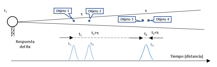
Where:
c is the speed of light.
τ is the pulse duration.
The factor 2 appears because the signal makes a round trip. A 1 µs pulse provides a range resolution of 150 m; a 2 µs pulse, 300 m; a 4 µs pulse, 600 m. A modern weather radar usually works between 150 and 250 m of range resolution using short pulses.dar meteorológico moderno suele trabajar entre 150 y 250 m de resolución radial mediante pulsos cortos.
Angular resolucion
It determines the ability to separate two targets located at the same range but positioned transversely to the optical axis of the antenna beam. It depends mainly on the beamwidth:
θ ≈ λ / D (it is an approximate value; a coefficient depending on the type of aperture must be included).
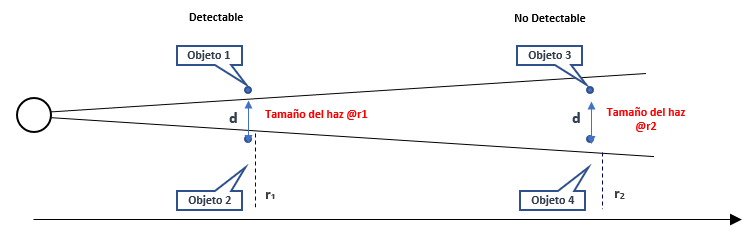
Where λ is the wavelength and D is the antenna diameter. A radar with a 1° beam has the following width depending on range:
| Range | Beamwidth |
|---|---|
| 50 km | 870 m |
| 100 km | 1.75 km |
| 200 km | 3.5 km |
This means that even if you have 150 m of range resolution, at 200 km the illuminated volume is several kilometers wide. What happens is that angular resolution worsens (in size) with range.
Volumetric resolution
n meteorology, what we actually measure is a volume. The resolution volume is approximated as:
V ≈ R² · θ² · ΔR
That is why the resolution volume increases rapidly with range. With a 1° beam and a range resolution of 250 m, at 50 km the volume is about 0.17 km³, but at 200 km it exceeds 11 km³. In other words, the same radar «sees» a cloud with much more detail nearby than far away. This is one of the fundamental limitations of radar observation.
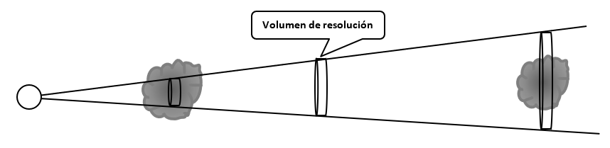
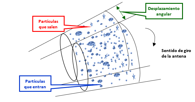
That resolution volume advances from the radar to the maximum range, returning toward the radar, CONTINUOUSLY, a signal that is the sum of the individual signals returned by each particle contained in that volume. Obviously, the radar cannot resolve anything inside that volume individually.
We do not know the number of particles, their composition (water, ice, or a mixture), their diameters, their shape, their orientation (if they are not spherical, for example ice crystals in the form of rods), or the speed and direction in which each one moves, nor do we know their position within the volume. We only have, at each instant of time, a sum signal (of the signals returned by each particle), which has an amplitude and a phase, resulting from the particles that volume is illuminating. One instant of time later, the volume will have moved a little along the optical axis of the antenna, and the signal will have changed according to the changes in the particles in the now-new volume.
The same process will happen with the next transmitter pulse, except that the antenna will have moved a little (a whole repetition period or more, for example, 1 millisecond), and therefore the particle composition will have changed more than what changes from one instant (1 microsecond, for example) to another along the same realization.
Each time the transmitter fires, we have a signal returned continuously in time, whose amplitude and phase vary according to the aforementioned configuration of the particles at each instant of time, and it extends to wherever we DETERMINE the working range should end.
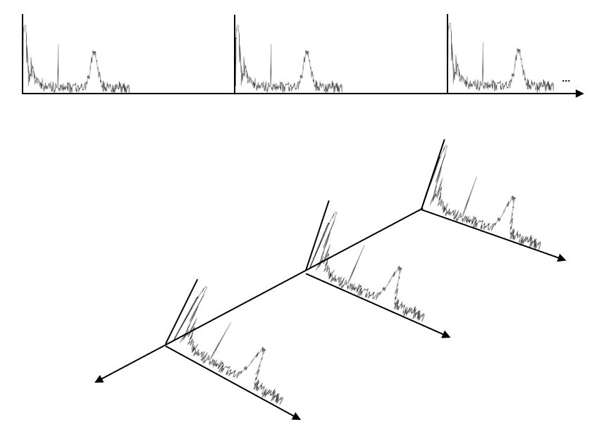
The transmitter pulse continues traveling through space and sending returned signals to the receiver, but we close the receiver and no longer «hear» beyond the limit we have set (150 km, 300 km, 500 km), whatever we have decided is reasonable.
Sampling and digitization
Normally, the radar user has little control over and influence on how close the samples taken along the same range are (unless they explicitly request it). This depends more on the capabilities of the signal processor (today, samples can be taken as close as 15 meters apart). Another element plays a role here: the processor’s ability to store samples (one thousand, 2 thousand, 4 thousand, 8 thousand memory cells), which is something that is constantly increasing and improving.
For example, if the processor capacity were one thousand samples, and you decide to sample at 15-meter spacing, the total range would reach only 15 km. To sample out to 500 km, it is not reasonable to take very small cell sizes even if the processor’s sampling speed allows it. For example, one thousand 500-meter cells would give us the desired 500 km.
Modern processors sample and digitize at the output of the receiver’s intermediate-frequency amplifier, and from then on the entire chain is digital. If you wish, read the post «Six generations of ingenuity: The evolution of signal processors in Cuban radars» (Seis generaciones de ingenio: La evolución de los procesadores de señal en los radares cubanos ) to understand how the matter of sampling evolved in processors, using the Cuban example.
In reality, the current capabilities of processors allow any desired sampling regime to be implemented; but one must have some notion of what makes sense and what does not. This brings us to the next point.
What resolution is needed, and for what?
Normally, clouds are several kilometers in size, so really, what would be the concern with resolution?
If the goal is to detect very small-scale phenomena — an incipient vortex within a supercell, a tornado signature, a localized convergence — the temptation is clear: the more resolution, the better. Small cells, fine grids, high-definition products. Anything that involves averaging or smoothing is perceived as a loss of potentially critical information. If you wish, read the post: «Can Doppler radars detect tornadoes?» (¿Pueden los radares Doppler detectar los tornados?)

But if the goal is to estimate precipitation and have those estimates resemble what rain gauges on the ground measure, things change. The reflectivity measured by the radar in a small volume is highly variable: drops of different sizes, distributions that change from one instant to another, beams that are not perfectly uniform. For the rainfall estimate to be representative of what falls in an area, it is better to average more, that is, use larger cells. The rain gauge integrates rainfall over an area and a time; the radar, if it wants to resemble it, also has to integrate.
There is the conflict: high resolution is good for not losing small vortices (in Doppler mode), but for precipitation it is better to increase the cell size to average more (in Reflectivity mode). It is not a black-and-white problem, but one of compromises. And to understand it well, we must separate two things that are often mixed: the radar’s resolution as a physical sensor, on the one hand, and the resolution of the acquisition cells and final products, on the other.
Something I must make clear regarding resolution:
No matter what resolution you sample at, you will NEVER see anything smaller than what the radar’s resolution volume allows for each range.
For many years, it was considered reasonably good to sample using polar cells of 1 km × 1 degree. From these polar cells, Cartesian products of 1×1 km², 2×2 km², or 4×4 km² were built. Certainly, why sample at sizes below the radar’s resolution if this will not lead to better resolution? The answer brings us to the next topic.
Signal fluctuation and improvement of estimates
The signal received at each instant of time is highly fluctuating, especially from one period to another; but also from one meter to another in range. If you wish, you can read this post for more details on signal fluctuation: «Why is the returned signal from a meteorological target so fluctuating?» (¿Por qué es tan fluctuante la señal retornada proveniente de un objeto meteorológico?).
Since these are fluctuating signals, it is necessary to filter that signal to obtain more precise estimates of Reflectivity, Velocity, and Spectral Width. This requires processing many samples, and it is desirable that these samples be statistically independent.
It was considered that if range samples were taken spaced, say, at 1 km, they would obviously be statistically independent, because it was enough to take them at distances greater than ΔR = (c · τ) / 2 for them to be so. Correct, but then the number of samples was small, and the reduction in the variance of the estimates was not so effective.
On the other hand, samples taken at the same range in successive periods are not statistically independent; one would have to let a large number of periods pass for them to be. Again, this yields few samples.
The slower the antenna moves and the higher the pulse repetition frequency, the more samples we obtain; but … in fast-moving atmospheric processes, such as tornadoes and downbursts (in Spain they call them «reventón»; in English, downburst), we cannot afford that luxury.
So, in my doctoral thesis, defended in 1999 but implemented in our signal processor starting in 1997 at the Camagüey radar, I proposed oversampling, that is, sampling below the size ΔR = (c · τ) / 2 and obtaining a larger number of samples, and I demonstrated that this contained statistically relevant information to improve the estimates.
Sebastián Torres’s thesis starts from this same oversampling idea outlined by me in the following work:
Rodriguez Gonzalez, O.L., 1999: Independent samples in range averaged finite bandwidth log receivers outputs. Preprints, 29th Conf. on Radar Meteorology, Montreal, Canada, Amer. Meteor. Soc., paper 10A.7.
He himself mentions me:
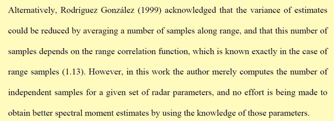
But Torres does the complete work, develops that idea to the end, proposing to apply a whitening transformation. In this way, those correlated samples (because they are taken at distances smaller than ΔR = (c · τ) / 2) are decorrelated, and by combining them in a weighted manner, an estimate with much lower variance is obtained. The benefit is twofold: the same precision in less scanning time, or greater precision while maintaining scanning time. That innovation led to super-resolution in NEXRAD radars.
We do not increase the number of samples to seek greater resolution, but to improve the statistics of the estimates (make them less fluctuating).
From polar cell to Cartesian pixel
So far we have talked about the resolution volume, the acquisition cells, and how fine sampling does not allow us to go beyond the radar’s instrumental resolution, the physical limit of the beam. But a question remains that is perhaps the most important for anyone looking at the screen: How do we go from those polar cells to the pixels we see in the final product?
Recall that the radar samples in polar coordinates: range, azimuth, and elevation. Each sample is an acquisition cell, and the set of all of them forms an image in polar coordinates. But most users do not see that raw image: we see a product on a Cartesian grid (x, y), like a map. That coordinate change is done through interpolation.
Each pixel of the Cartesian grid is not a direct radar measurement. It is a weighted combination of several neighboring polar cells. Depending on the product cell size and the range to the radar, a pixel may be formed by a single polar cell or by several. Near the radar, where the polar cells are small, a 1 km × 1 km pixel can contain many cells. Far away, where the resolution volume is already several kilometers, a 1 km × 1 km pixel can be smaller than a single polar cell: in that case, the interpolation is not creating information, it is only oversampling.
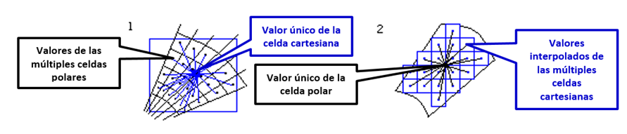
Here is the key: the product cell size is a user decision, not a physical consequence. We can have data acquired with 250 m cells and generate 1 km, 500 m, or 2 km products. And that decision has consequences. In the VESTA system, something more absurd can be done: acquire data in 1 km cells and generate 250 m or 500 m products (or any other value you can think of).
If we choose small product cells, we better preserve fine structure: a small vortex, an echo edge, a localized convergence, the abrupt boundary of hail. But we also preserve more noise. The radar signal is fluctuating, and small cells do not average enough to stabilize the estimate. The result is more detailed but more «speckled» products.
If we choose large product cells, we smooth more. The estimate is more stable, more similar to what a rain gauge integrates, but we lose the ability to see small-scale phenomena. A distant tornado can disappear inside a pixel that is too large.
For many years, the standard was to sample in polar cells of 1 km × 1° and generate Cartesian products of 1 km × 1 km, 2 km × 2 km, or 4 km × 4 km. It was not an arbitrary choice: at medium ranges, the resolution volume was already of that order, and it did not make much sense to generate finer products than the original data. With the arrival of super-resolution and more powerful processors, that standard has been refined: today it is possible to acquire with 75–150 m cells and generate 500 m or even 250 m products, at least near the radar.
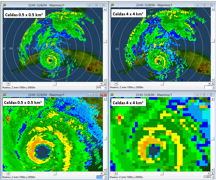
But we should not fool ourselves. Interpolating does not create information. If the resolution volume at 150 km already has a transverse width of 2 km, a 500 m product will not show us more real detail: it will only show us a smoothed version of the same information, but with more pixels. The effective resolution of the product can never be better than the effective resolution of the data.
So, what does each pixel represent? It represents an estimate of reflectivity, velocity, or spectral width, averaged over a volume that changes with range and angle. It is not a point measurement. It is not a photograph of the atmosphere. It is a weighted integration of what is inside a resolution volume, and that volume grows with range.
The next time you look at a radar image, ask yourself: What is inside that pixel? Is it a small, intense cell or a large, moderate cell? Am I seeing real detail or the result of interpolation? The answer is not always simple, but the mere fact of asking it makes you a more conscious user of what the radar can and cannot tell you.
References
- Torres, S.M. (2001). Estimation of Doppler and polarimetric variables for weather radars. PhD Dissertation, University of Oklahoma.
- Rodriguez Gonzalez, O.L. (1999). Independent samples in range averaged finite bandwidth log receivers outputs. Preprints, 29th Conf. on Radar Meteorology, Montreal, Canada, Amer. Meteor. Soc., paper 10A.7.
- Doviak, R.J., & Zrnic, D.S. (1993). Doppler radar and weather observations. Academic Press.
- Bringi, V.N., & Chandrasekar, V. (2001): Polarimetric Doppler Weather Radar.
- Rinehart, R.E. (2004): Radar for Meteorologists.
- Torres, S., & Curtis, C.D. (2015). Design considerations for improved tornado detection using super-resolution data on the NEXRAD network.
- NOAA/NWS. Radar Fundamentals.
- Radartutorial.eu. Capítulos de Range Resolution, Beamwidth, Pulse Compression y Doppler Processing.
Deja una respuesta